During my first academic term, I have completed a final assignement and for the topic I have chosen to focus on the banking sector and the issues of credit risk assessment. I conducted an analysis of an open database from a repository of Chief Data Scientist at Prediction Consultants in Israel - Roi Polanitzer (github account). The raw data can be found here. Here you may find my visualization for othe case of Credit Risk. I conducted an analysis of an open database from The Kaggle.com. The data source is here.
Content
Problem and dataset
Problem formulation
Over the past four decades, there has been a consistent increase in the share of household loans and debts in GDP across most countries, highlighting the significance of credit as a reliable financial instrument according to International Monetary Fund statistic (2022).
Banks offer a wide range of credit services, with loans being a primary source of income (Miguéis V.L., Benoit D.F. and Van den Poel D. 2013). To ensure a steady flow of credit payments and avoid profit loss, banks must assess clients’ credit risk. Researchers have explored Machine Learning techniques to develop accurate credit risk assessment models, leading to promising methods for evaluating default probabilities (Florez-Lopez R. and Ramon-Jeronimo J.M. 2014, Hooman A. et al 2016). The researchers Subburayan B. et al emphasize the inevitability of the transformation of the banking sector with the help of Machine Learning (2023).
The transformation of the banking sector through Machine Learning is emphasized, impacting areas such as quality assessment, transaction trends, and customer satisfaction, thereby enhancing customer happiness and income. Effective risk management is crucial in banking operations, improving loan portfolios, reducing credit losses, and lowering default rates. Implementation of risk-driven approaches based on Machine Learning can yield time-saving solutions and address big data challenges, with potential reputational and financial benefits.
Despite having limited information, banks must ensure the reliability of their data to develop tailored methods for assessing credit risks. From all this it follows that banks face an important problem: how to assess the credit risk for each new customer with information about their default experience? My work provides one of possibles answer to this question.
Dataset description
This research is based on a dataset extracted from a Roi Polanitzer’s github repository. It contains 41188 samples with 9 features. These features are:
- age – customer age, years;
- education – customer education level;
- years_with_current_employer – time with current employer, years;
- years_at_current_address – time at the current address, years;
- household_income – annual income, in thousands of USD;
- debt_to_income_ratio – debt-to-income ratio, %;
- credit_card_debt – debt on the credit card, in thousands of USD;
- other_debt – other debts, in thousands of USD;
- y – indicates whether a customer defaulted in the past if = 1 than yes, if = 0 does not.
The analysis is based on the hypothesis that unpaid debts in the past leads to unpaid debts in the future. That is why the ‘y’ variable is dependent in the models in this project. Moreover, it presents two classes of customers: reliable if ‘y’=0 and unreliable if ‘y’=1.
All further calculations are made in Python. The data is partly presented below.
Dataset transforming
A few steps are made in order to detect errors and inaccuracies and as a result having clean data for further analysis.
- to detect Nan values;
- to detect abnormal values;
- to check all values are with expected type.
print(dataset.head())
Output
| # | loan_applicant_id | age | education | years_with_current_employer | years_at_current_address | household_income | debt_to_income_ratio | credit_card_debt | other_debt | y |
|---|---|---|---|---|---|---|---|---|---|---|
| 0 | 191 | 44 | university.degree | 10 | 20 | 192 | 12.116645 | 14.377313 | 8.886645 | 1 |
| 1 | 34318 | 34 | high.school | 3 | 18 | 57 | 14.264229 | 5.137880 | 2.992730 | 0 |
| 2 | 14932 | 45 | university.degree | 14 | 24 | 212 | 7.285681 | 10.460306 | 4.985339 | 0 |
| 3 | 2776 | 33 | illiterate | 12 | 5 | 418 | 11.386272 | 3.040189 | 44.554429 | 1 |
| 4 | 11915 | 20 | basic | 4 | 19 | 122 | 28.418494 | 14.560450 | 20.110112 | 0 |
No significant errors or missing values were found. If any were discovered, they can be replaced using one of the following methods: 1) Completely removing such objects from the data set (I do not recommend this method); 2) Replacing each value with the mean of the sample.
print(dataset.info())
Output
    <class 'pandas.core.frame.DataFrame'>
RangeIndex: 41188 entries, 0 to 41187
Data columns (total 10 columns):
 #   Column                       Non-Null Count  Dtype
---  ------                       --------------  -----
 0   loan_applicant_id            41188 non-null  int64
 1   age                          41188 non-null  int64
 2   education                    41188 non-null  object
 3   years_with_current_employer  41188 non-null  int64
 4   years_at_current_address     41188 non-null  int64
 5   household_income             41188 non-null  int64
 6   debt_to_income_ratio         41188 non-null  float64
 7   credit_card_debt             41188 non-null  float64
 8   other_debt                   41188 non-null  float64
 9   y                            41188 non-null  int64
dtypes: float64(3), int64(6), object(1)
memory usage: 3.1+ MB
It is seen that the database contains 41,188 records. This is a significant amount from which to draw representative conclusions. All the data is in the expected format. At the same time, I have a desire to standardize the “education” feature. It is made as:
def educational_coding(dataset):
    education_mapping = {
        'university.degree': 1,
        'high.school': 2,
        'illiterate': 3,
        'basic': 4,
        'professional.course': 5
    }

    dataset['education'] = dataset['education'].replace(education_mapping)
    return(dataset)
Dataset statistics
Now, let us take a look at some descriptive statistics to form the big picture of the database:
print(dataset.describe().to_string())
Output
Whole dataset description
              age  education  years_with_current_employer  years_at_current_address  household_income  debt_to_income_ratio  credit_card_debt  other_debt
count  41188.000  41188.000                    41188.000                 41188.000         41188.000             41188.000         41188.000   41188.000
mean      38.008      2.993                       13.550                    15.385           139.707                16.224             9.577      13.758
std       10.624      1.419                        8.145                     9.184            81.688                 9.191            12.409      14.597
min       20.000      1.000                        0.000                     0.000            14.000                 0.400             0.006       0.022
25%       29.000      2.000                        6.000                     7.000            74.000                 8.452             1.853       3.784
50%       38.000      3.000                       14.000                    15.000           134.000                16.105             5.311       9.154
75%       47.000      4.000                       21.000                    23.000           196.000                23.731            12.637      18.907
max       56.000      5.000                       29.000                    31.000           446.000                41.294           149.016     159.198
The boolean value of Y can be ignored, since statistics do not provide any useful information. This value is analysed later. I drawn a portrait of an average bank customer. He/she is 38 years old and most likely illiterate, also he/she has not changed jobs in 13 years and has been living in the same place for more than 15 years. The average salary is $139,700 per year, but about 16% of that amount is in debt, including about $9,600 in credit card debt and $13,800 in other debt.
The median (50%) also indicates that the variables are mostly evenly distributed, while for credit_card_debt and other_debt the average is shifted to the second half of the dataset.
I assume that function ‘describe()’ provides not enough details, and I decided to create its own table with more coefficients: Harmonic Mean, Range, Mode, Skewness, Kurtosis.
Output
                         age  education  years_with_current_employer  years_at_current_address  household_income  debt_to_income_ratio  credit_card_debt  other_debt
Harmonic Mean        34.830      2.178                        0.000                     0.000            82.480                 7.525             1.172       3.149
Range                36.000      4.000                       29.000                    31.000           432.000                40.894           149.010     159.176
Mode                 43.000      1.000                        2.000                    28.000           201.000                12.117            14.377       8.887
Skewness              0.002      0.003                        0.015                     0.004             0.759                 0.148             3.279       2.558
Kurtosis             -1.206     -1.307                       -1.192                    -1.199             0.910                -0.875            16.972      10.950
- Harmonic Mean is very different from the Mean for household_income, debt_to_income_ratio, credit_card_debt, and other_debt. This indicates that there are extreme values in the data. If Harmonic Mean = 0, means there is a zero value in the data, so, cannot say anything about the difference for such variables.
- Range and Standard Deviation together clearly indicate that there is a significant variation in the data. I believe this is because of the large number of objects which represent different groups of people.
- Mode shows the most common values. They are seen from the table, does not require lots of comments
- Skewness is close to zero, which indicates that there is no significant asymmetry in the distribution of education levels. Except for household_income, credit_card_debt, and other_debt it is positive and above zero, meaning the data distribution shows a right-skewed asymmetry, which means there is a longer tail on the right. This is typical of financial indicators, in which there are no upper limits on values. For example, there is an age limit and, accordingly, a time limit for living/working at one location.
- Kurtosis also mostly have a very big and negative number, means the curves are more flatter vertices and lighter tails. Household_income, credit_card_debt, and other_debt have high sharp peaks and long outliers.
Visualization
To learn more about the behavior patterns within reliable and unreliable customers, the metrics of these two groups is considered. Moreover, number of observations in a group of reliable clients (Y=0) is almost 8 times more than in an unreliable one (Y=1).
Value 'y'
0    36548
1     4640
Name: count, dtype: int64
Next, two groups of data are analyzed separately, and their descriptive statistics are presented further. In short, the means and standard deviation values between groups are the same, except for the group of clients with debt. For them the indicators are significantly higher.
Dataset of reliable clients description
print(dataset_0.describe().to_string())
Output
              age  education  years_with_current_employer  years_at_current_address  household_income  debt_to_income_ratio  credit_card_debt  other_debt
count  36548.000  36548.000                    36548.000                 36548.000         36548.000             36548.000         36548.000   36548.000
mean      37.976      2.995                       13.448                    15.498           128.301                15.515             7.811      12.127
std       10.686      1.420                        8.063                     9.246            66.318                 8.665             8.427      11.344
min       20.000      1.000                        0.000                     0.000            14.000                 0.400             0.006       0.022
25%       29.000      2.000                        6.000                     7.000            71.000                 8.041             1.651       3.552
50%       38.000      3.000                       13.000                    16.000           128.000                15.530             4.724       8.480
75%       47.000      4.000                       20.000                    24.000           186.000                22.935            11.126      17.334
max       56.000      5.000                       27.000                    31.000           242.000                30.600            55.344      68.666
Dataset of unreliable clients description
print(dataset_1.describe().to_string())
Output
             age  education  years_with_current_employer  years_at_current_address  household_income  debt_to_income_ratio  credit_card_debt  other_debt
count  4640.000   4640.000                     4640.000                  4640.000          4640.000              4640.000          4640.000    4640.000
mean     38.261      2.980                       14.356                    14.500           229.555                21.810            23.490      26.605
std      10.112      1.411                        8.723                     8.637           124.487                11.109            24.277      26.302
min      21.000      1.000                        0.000                     0.000            14.000                 2.407             0.057       0.222
25%      29.000      2.000                        7.000                     7.000           122.000                12.293             5.807       7.537
50%      38.000      3.000                       14.000                    15.000           231.000                21.831            14.528      17.818
75%      47.000      4.000                       22.000                    22.000           336.000                31.244            33.632      36.710
max      55.000      5.000                       29.000                    29.000           446.000                41.294           149.016     159.198
Histogram of the distribution frequency
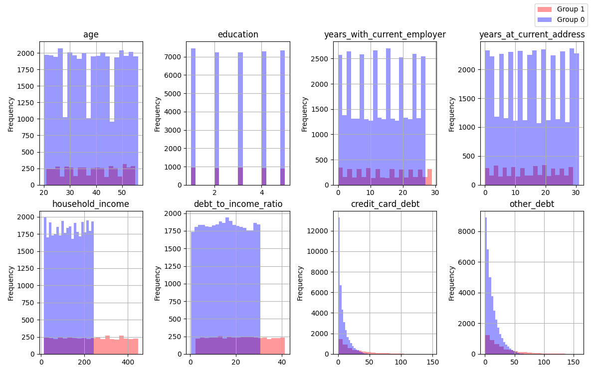
From the histogram of the frequency distribution, it can be seen that Group 1, which includes unreliable customers (those who were previously identified as defaulting), is clearly inferior in terms of number. It’s interesting to note that these clients tend to have household incomes above $220,000. And at the same time, many of them have a significant amount of debt on credit cards and other sources. Based on this information, I can assume that among these unreliable clients, there are a significant number of people who earn more than average and, at the same time, use borrowed funds, and these amounts also exceed average levels.
Distribution density diagram
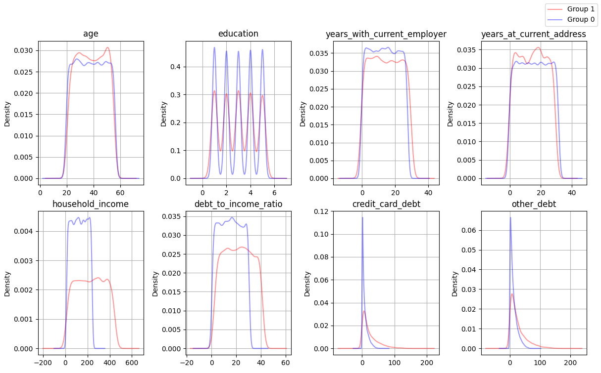
Density diagrams clearly show that, for income and debts ratio, the expected values are higher for unreliable customers. There is a greater spread of data or the presence of outliers for these features. I have also noted that the distributions of credit card debt and other types of debt are not very similar. The figure also correspond with the description of Skewness and Kurtosis mentioned above.
Now let’s move on to analyzing the strength and nature of the relationship between the parameters. For these purposes, a matrix of correlations between all parameters has been calculated. It is interesting to observe how the parameters influence the dependent variable - ‘Y’. However, it is not feasible to do this individually for each group, as ‘Y’ does not vary (for all customers ‘Y’ is either 0 or 1).
Correlation matrix for the whole dataset
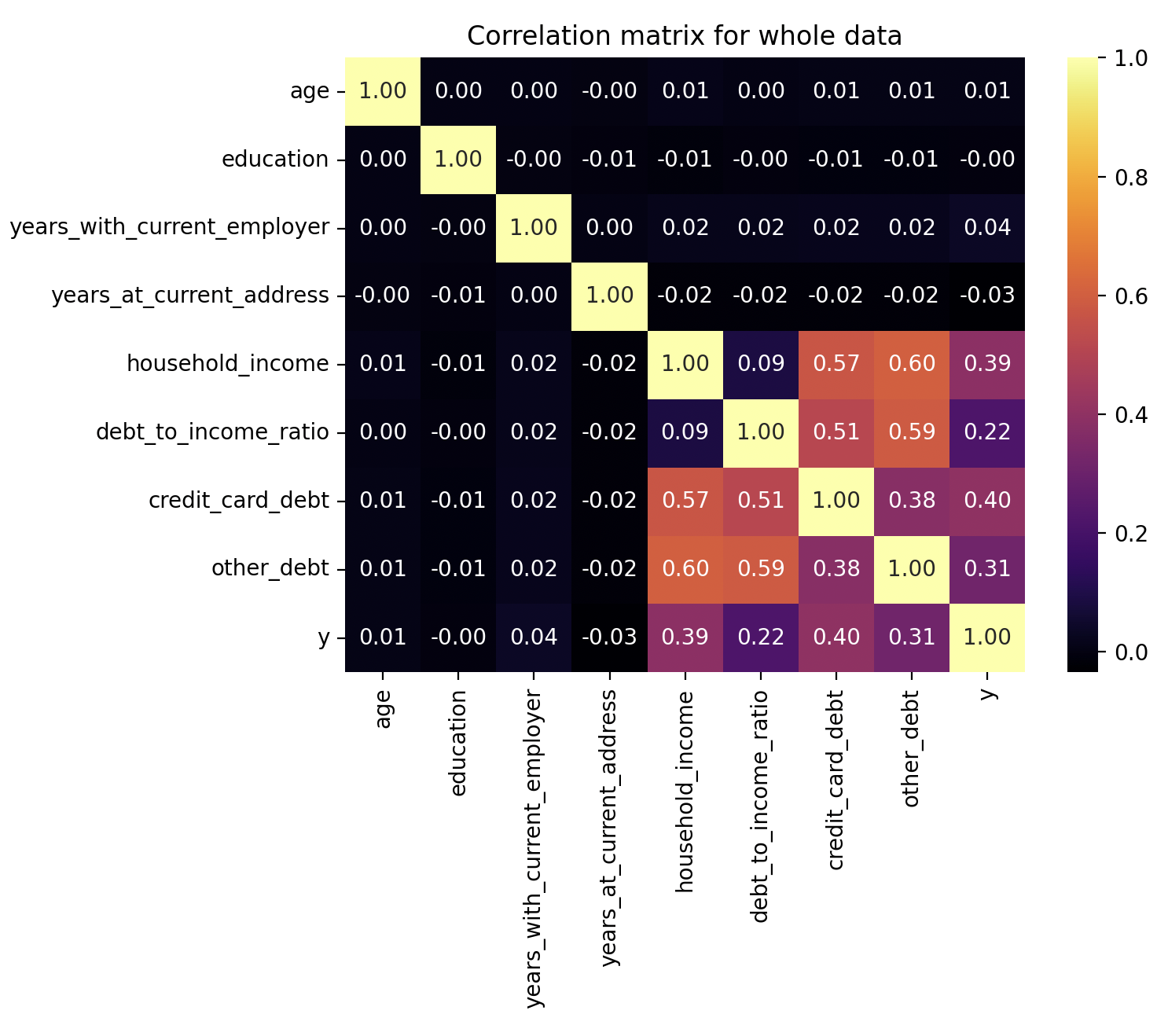
Due to the large data set, it is clear which parameters significantly affect the independent variable. Income growth is associated with an increase in debts and the debt-to-income ratio. However, I am not entirely sure what exactly causes people to take out loans when their income increases. Maybe some individuals are business owners who find it normal to use credit for working capital purposes. Or, perhaps it is a household where, despite rising income, the needs increase faster, for instance, due to the need for expensive purchases such as large houses, cars, or expensive educations for children.
In summary, the main indicator, is the debt to income ratio. The greater the proportion, the greater the likelihood that the customer will not repay the debt.
Models implementation
For the classification task Logistic regression is chosen. It works well on large datasets. It is also easy to interpret, and can predict the probability of belonging to a class, which is useful for decision-making. The second excellent method is the K-Nearest Neighbors. Unfortunately, it is difficult to identify whether the studied data have linear dependency, so the method deals well with nonlinear dependencies between features and the target variable. On the other hand, the method may be less effective on large datasets. Despite this, it is worth trying to evaluate both models.
The following Python libraries are used to program the modelss: train_test_split, StandardScaler, LogisticRegression, and KNeighborsClassifier.
Logistic regression model
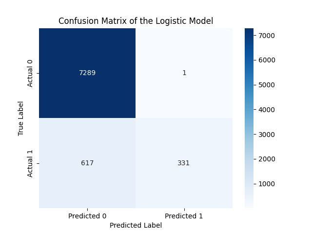
The model was trained on 80% of the dataset and then evaluated. The accuracy is quite high, equal to 92%. This I consider to be an excellent indicator of the model’s performance. The precision and recall scores are also quite good, but the ability of the model to identify unreliable customers (Class 1) is not that good. Only 35% of these customers were correctly identified by the model. I believe this is due to the imbalance in the distribution of data between classes. I have tried using the class weighting technique to address the issue, but the accuracy and other indicators have actually worsened in some cases.
def log_reg(X_train, X_test, y_train, y_test):
    model = LogisticRegression(max_iter=5000)
    model.fit(X_train, y_train)
    predictions_train = model.predict(X_test)
    print("\nClassification Report for the Logisic Rergession:\n",
          classification_report(y_test, predictions_train))
    conf_matrix_log_reg = confusion_matrix(y_test, predictions_train)
Model assessment
Classification Report for the Logisic Rergession:
               precision    recall  f1-score   support
           0       0.92      1.00      0.96      7290
           1       1.00      0.35      0.52       948
    accuracy                           0.92      8238
   macro avg       0.96      0.67      0.74      8238
weighted avg       0.93      0.92      0.91      8238
Confusion matric for the Logistic regression
Random Forest model
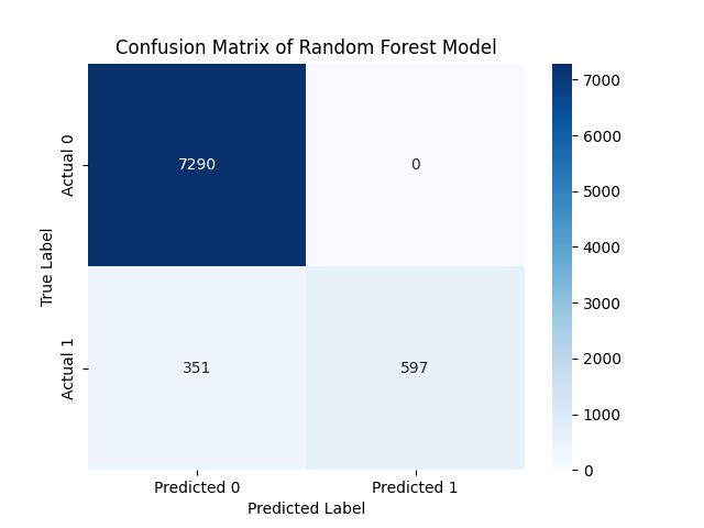
The model was trained on 80% of the dataset and then evaluated. The accuracy is even higher, equals to 96%. All indicators of the model have improved, and it now recognizes a smaller group even better.
    model_rf = RandomForestClassifier(n_estimators=n_estimators,
                                      random_state=42)
    model_rf.fit(X_train, y_train)
    y_pred_rf = model_rf.predict(X_test)

    print("Classification Report for the Random Forest:\n",
          classification_report(y_test, y_pred_rf))

    cm = confusion_matrix(y_test, y_pred_rf)
Model assessment
Classification Report for the Random Forest:
              precision    recall  f1-score   support
           0       0.95      1.00      0.98      7290
           1       1.00      0.63      0.77       948
    accuracy                           0.96      8238
   macro avg       0.98      0.81      0.87      8238
weighted avg       0.96      0.96      0.95      8238
Confusion matric for the Random Forest
Predictions
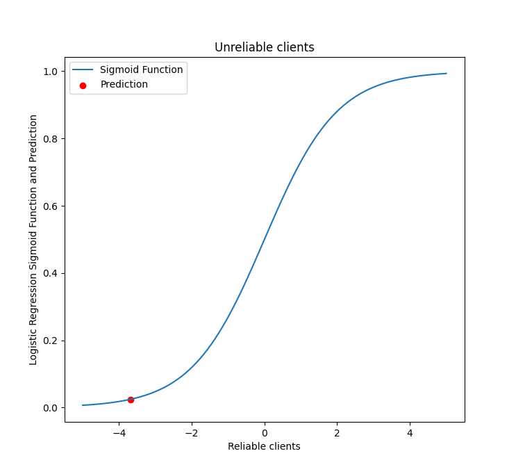
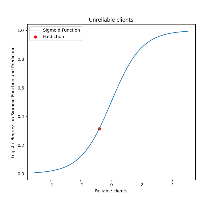
Trained models can be used to determine whether a new client will be reliable and repay the loan, or not. The bank should not provide a loan to such clients. Consider the example of two clients. Please, see the table below.
Based only on the descriptive statistics of the data, it is already possible to assume that the Second client is more likely to get the credit from a bank than the first client, since his debt to income ratio tends towards the average value for reliable clients. However, in order to be sure, it is necessary to make a prediction based on the models.
There are the results!
| Parameter | First Client | Second Client |
|---|---|---|
| Age | 58 | 31 |
| Education | 2 (High School) | 5 (Professional Course) |
| Years with Current Employer | 24 | 2 |
| Years at Current Address | 3 | 4 |
| Household Income | 59.6 | 159.6 |
| Debt-to-Income Ratio | 15.00 | 36.66 |
| Credit Card Debt | 3.58 | 23.4 |
| Other Debt | 5.36 | 35.12 |
| Logisic Rergession | Predicted class = [0] | Predicted class = [0] |
| Random Forest | Predicted class = [0] | Predicted class = [1] |
For the first client, the class was assigned in the same way for both models. To illustrate the difference between the two models, let’s take a look at the assigned class and probability in logistic regression.
The example of the second client demonstrates that if it is challenging to uniquely identify a customer in one of the groups using one of the approaches, then it may be beneficial to employ a combination of both methods.
In more details
# Content 1. [Key findings](#title1) 2. [Management recommendations](#title2) 3. [Concluding remarks](#title3) The probability of not repaying the loan was extremely low, equal to just 1.93%. You can see this on the sigmoind function above. Meanwhile, the probability was much higher for the second client = 31.40%. Even so, the client can still be trusted to make payments. However, the random forest model treated this client more strictly, classifying them as an unreliable customer.Sigmoid function for the first (left) and the second (right) client
Concluding remarks
After the analysis, the main findings can be practically applied in the Artificial Bank operation. In particular, the distinctive characteristics of reliable and unreliable groups, as well as the main factors influencing group belonging.
- Firstly, to use the proposed model in the web application on daily basis for decision making. Just entering the client’s basic data, such as age, education level, work experience, residence at the same address, annual income, debt-to-income ratio, credit card and other debts, and the probability of being unreliable is calculated.
- Secondly, to design its own credit scores, for example, the “ABC” system, dividing customers into three groups depended on the probability of being unreliable. Group “A” includes the most reliable clients (0.45–0), “C” - the least reliable (1–0.56), and “B” (0.55–0.46) is considered a “Gray zone” where changes are required to improve the assessment, for example, an find new income sources or repayment of existing debts.
- Thirdly, to supplement the database with new loan parameters to improve the model such as term, interest rate, and amount. It may extend the model. To improve the model, I recommend a more in-depth analysis of the influence of the debt structure, the income of all members of the household, and household composition. Additionally, as a new factor, I would like to consider the impact of a credit terms on the final decision-making process. This could be assisted by statistics on the following factors: total amount, duration, purpose, and the percentage of the requested credit.
These recommendations may reduce the percentage of non-repayment loans and increase the bank’s assets turnover, making it more financial stable.
Thank you for your attention. I am available to answer any questions or provide suggestions
Bibliography
- Florez-Lopez R. and Ramon-Jeronimo J.M. (2014) ‘Modelling credit risk with scarce default data: on the suitability of cooperative bootstrapped strategies for small low-default portfolios.’ The Journal of the Operational Research Society 65 (3) 416-434
- Hooman A. et al (2016) ‘Statistical and data mining methods in credit scoring.’ The Journal of Developing Areas 50 (5) 371-381
- International Monetary Fund (2022) Household debt, loans and debt securities [online] available from https://www.imf.org/external/datamapper/HH_LS@GDD/CAN/GBR/USA/DEU/ITA/FRA/JPN/VNM. [25 January 2024]
- Miguéis V.L., Benoit D.F. and Van den Poel D. (2013) ‘Enhanced decision support in credit scoring using Bayesian binary quantile regression.’ The Journal of the Operational Research Society 64 (9) 1374-1383
- Subburayan B. et al (2023) Patent - Transforming Traditional Banking The AI Revolution Research Gate [online] available from https://www.researchgate.net/publication/374504440_Patent__Transforming_Traditional_Banking_The_AI_Revolution/.> [20 January 2024]
- Witzel M., and Bhargava N. (2023), ‘AI-Related Risk: The Merits of an ESG-Based Approach to Oversight.’ Centre for International Governance Innovation